Linearized Rossby wave model

This page works as an example of how the basic linear rossby model works and how to interpret and play with it. The first step is to import the necessary libraries including qg_model numpy and matplotlib

import qg_model as qg
import numpy as np
import matplotlib.pyplot as plt

Set up the model

The model works as an opensource code, so is possible to review the code to have a better understanding of everything that’s going on behind it. In this case to initialize the model, this requiere the following inputs:

• duration: Indicates de number of days that you want the model to run.

• dt: Indicates the length of each time step.

• xmax: Indicates the maximun number in the x axis

• ymax:Indicates the maximun number in the y axis

• lat: Refers to the latitude in which the calculation will take place

m=qg.barotropic_models(duration=10,dt=7200,lat=45,xmax=256,ymax=256)

Running the model

The function snapshot_generator() works in two ways, running the model and generating the snapshots. Since the model goal is to show the time evolution of the vorticity, is necessary for us to generate snapshots while in the process, this procedure will let us see how the vorticity behaves as time moves forward. It is important to remember that the Barotropic vorticity equation is solved through Adams-Bashford time stepping scheme, this means that every time step refers to a state of the Vorticity or more convenient to us a snapshot.

pv_snap=m.snapshot_generator()

---------------------------------------------------------------------------
KeyboardInterrupt                         Traceback (most recent call last)
Input In [3], in <cell line: 1>()
----> 1 pv_snap=m.snapshot_generator()

File ~/openqg/book/qg_model.py:171, in barotropic_models.snapshot_generator(self, tsnapstart, tsnapint)
    168 nt = np.ceil(np.floor((tmax-tsnapstart)/self.dt+1)/tsnapints).astype('int')
    169 pv_snap=np.zeros((self.xmax,self.ymax,nt),dtype=complex)
--> 171 for snapshot in self.run():
    172     pv_snap[:,:,tind]=self.DFFT_Back(self.q[:,:,3])
    173     tind=tind+1

File ~/openqg/book/qg_model.py:144, in barotropic_models.run(self)
    142             self.adv_q[i,j,0] = self.adv_q[i,j,1]
    143         # run the tendency
--> 144         self.q[i,j,3] = self.q[i,j,2] +self.dt*(23.0*self.adv_q[i,j,2]-16.0*self.adv_q[i,j,1]+5.0*self.adv_q[i,j,0])/12.0
    145 # swap
    146 for i in range(1,self.mmax):

KeyboardInterrupt: 

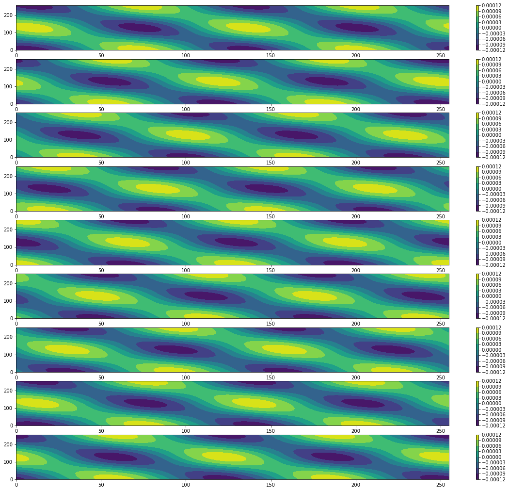
Model output

Every snapshot that comes out of the model can be later on ploted in order to see time evolution of the Vorticity, in this case the model is set to return a snapshot every 10 steps. The picture below show the points of negative and positive vorticity, which in these case is fully dependent of the flow direction. Also the shape of the vortix is related to initial perturbations that the model takes.

plt.figure(1)
fig = plt.gcf()
fig.set_size_inches(20, 20)
#fig.savefig('test2png.png', dpi=100)

for i in range(1,10):
    plt.subplot(10,1,i)
    plt.contourf(np.real(pv_snap[:,:,i]).T)  
    plt.colorbar()

plt.show()

Animation

It is possible to see the evolution of the Barotropic vorticity with the function snapshot_animation() which makes a recopilation of every snapshot to plot it as time advances. In the following animation, we can see that infact the rossby waves move westwards